The world is not flat, it’s highly nested
With over 4 billion page views per day and over 100TB of data collected daily, scale at Taboola is no joke. Our primary data pipe deals with masses of data and endless read paths. Could we optimize our schema for all these read paths? Guess not…
Our schema is HUGE and highly nested.
After digesting the data, we keep it in hourly Parquet files on HDFS, where each hour consists of about 1-1.5TB of compressed data.
Our schema roughly looks like this:
root
|-- userSession: struct
| |-- maskedIp: long
| |-- geo: struct
| | |-- country: string
| | |-- region: string
| | |-- city: string
| |-- pageViews: array
| | |-- element: struct
| | | |-- url: string
| | | |-- referrer: string
| | | |-- widgets: array
| | | | |-- element: struct
| | | | | |-- name: string
| | | | | |-- attributes: map
| | | | | | |-- key: string
| | | | | | |-- value: string
| | | | | |-- recommendations: array
| | | | | | |-- element: struct
| | | | | | | |-- slot: integer
| | | | | | | |-- type: string
| | | | | | | |-- campaign: long
| | | | | | | |-- clicked: boolean
| | | | | | | |-- cpc: decimal(10,4)
It contains over a thousand columns, with repeated fields and maps interwound together.
Parquet is a columnar format, allowing one to query for a certain nested column without reading the entire structure containing it. So in the example above, one could execute the following query without fetching the entire userSession data to the client:
select userSession.geo.city from user_sessions
We use Spark widely to produce reports, carry out our billing process, analyze A/B tests results, feed our Deep Learning training processes and much more.
But Spark turned out to be crude when pruning nested Parquet schemas. It surprised us to see that running the above query in Spark SQL would result in reading the entire data into Spark executors. Redundant fields are omitted only on client side, leaving us with the required fields for the query (highlighted):
root
 |-- userSession: struct
 |    |-- maskedIp
 |    |-- geo: struct
 |    |    |-- country: string
 |    |    |-- region: string
 |    |    |-- city: string
 |    |-- pageViews: array
 |    |    |-- element: struct
 |    |    |    |-- url: string
 |    |    |    |-- referrer: string
 |    |    |    |-- widgets: array
 |    |    |    |    |-- element: struct
 |    |    |    |    |    |-- name: string
 |    |    |    |    |    |-- attributes: map
 |    |    |    |    |    |    |-- key: string
 |    |    |    |    |    |    |-- value: string
 |    |    |    |    |    |-- recommendations: array
 |    |    |    |    |    |    |-- element: struct
 |    |    |    |    |    |    |    |-- slot: integer
 |    |    |    |    |    |    |    |-- type: string
 |    |    |    |    |    |    |    |-- campaign: long
 |    |    |    |    |    |    |    |-- clicked: boolean
 |    |    |    |    |    |    |    |-- cpc: decimal(10,4)
In this scenario, given that the other elements in the schema are repeated, we may very well end up throwing away 99% of the data that we fetched from Parquet.
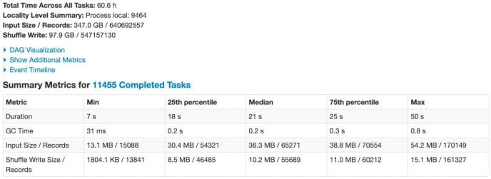
Image 1 depicts the total input size and execution time for one of our actual (but not heaviest) queries in production. It reads into Spark about 350GB (out of 1.1TB of hourly data).
Total time across all tasks: ~60h, with 36MB input per task on median.
Image 1: stats for stage reading input for production query
Prune it yourself
We decided to make it easier on Spark, and “flatten” our schema as much as possible. That is – prune any nesting level for non repeated or map fields.
So our above example schema then looked like this:
root
 |-- userSession_maskedIp: long
 |-- userSession_geo_country: string
 |-- userSession_geo_region: string
 |-- userSession_geo_city: string
 |-- userSession_pageViews: array
 |    |-- element: struct
 |    |    |-- url: string
 |    |    |-- referrer: string
 |    |    |-- widgets: array
 |    |    |    |-- element: struct
 |    |    |    |    |-- name: string
 |    |    |    |    |-- attributes: map
 |    |    |    |    |    |-- key: string
 |    |    |    |    |    |-- value: string
 |    |    |    |    |-- recommendations: array
 |    |    |    |    |    |-- element: struct
 |    |    |    |    |    |    |-- slot: integer
 |    |    |    |    |    |    |-- type: string
 |    |    |    |    |    |    |-- campaign: long
 |    |    |    |    |    |    |-- clicked: boolean
 |    |    |    |    |    |    |-- cpc: decimal(10,4)
As you can see, if one wants to query now for the city column, Spark doesn’t need to read the entire data, only the queried column will be read.
But what if we wanted to compute the revenue (the sum of cpc for all clicked items)? We still had to read a lot of data, the entire userSession_pageViews instead of the fields participating in the Spark SQL query below.
select sum(rec.cpc) from user_sessions
lateral view explode (userSession_pageViews) as pv
lateral view explode (pv.widgets) as widget
lateral view explode (widget.recommendations) as rec
where rec.clicked = true
We came across the notorious SPARK-4502 bug. Though there was an open pull request for this, it was not progressing as quickly as we needed…
We realized that if we provided Spark with the required schema, making it “blind” to the unnecessary payload, we could reduce input size for our queries. We tried it for a couple of queries and it showed promising results. We even used it in production for our heaviest queries, providing the schema manually. But with dozens (and nowadays hundreds) of routine queries, we realized manual pruning just wouldn’t scale.
Giving it our best effort
While the heroic thing to do was to buckle down and help with Spark PR, there were few reasons to take a different course of action:
- It’s still out of our hands – months could still go by until the issue is fixed in some future Spark version, along with all of the risks involved in upgrading.
- Even if a fix was slated to be released, we didn’t want to constrain ourselves to upgrading. We have a mono repo with multiple services and different use cases, and upgrading is challenging (but that’s for another post).
We decided to tackle it from a different angle, one that is based on the fact that Spark is using lazy evaluation, and so we developed ScORe (open source) for Spark SQL queries.
Given any Spark SQL query, we can take its logical plan, and gauge which columns from the underlying data source are participating in it. We can then create the required schema, and then recreate the dataframe with the schema that we generated. It is only then that we perform any action.
So we basically take the original (full) schema, and try to nail the perfect ScORe (schema on read) out of it.
Traverse the woods
Deriving the required schema for a Spark SQL query starts with passing the LogicalPlan of the query to SchemaOnReadGenerator.
The examples in this section will assume the following schema:
root
 |-- nestedStruct: struct
 |    |-- childStruct: struct
 |    |    |-- col1: long
 |    |    |-- col2: long
 |    |-- str: string
 |-- someLong: long
 |-- someStr: string
Simple Enough
Let’s consider the following Spark SQL query:
df.select(“someLong”, “someStr”)
.filter(“someLong = 5”)
.select(“someStr”)
You probably noticed that the query is very simple, over top level columns. This would help us understand how ScORe works, and later on we’ll get into a more complex example.
Back to our query. This is what the logical plan looks like:
'Project [unresolvedalias('someStr, None)]
+- Filter (someLong#52L = cast(5 as bigint))
   +- Project [someLong#52L, someStr#53]
      +- Relation[nestedStruct#46,someArrayOfArrays#47,someArrayOfComplexArrays#48,someBoolean#49,someComplexArray#50,someDouble#51,someLong#52L,someStr#53,someStrArray#54,struct#55] parquet
A LogicalPlan is a TreeNode object. Each TreeNode contains a sequence of TreeNode children, and according to its concrete type class, other properties.
For instance, the Project is by itself a LogicalPlan, having a single child LogicalPlan, and a ProjectList.
In our example, the ProjectList contains `someStr`, and the child LogicalPlan is the Filter.
We iterate over the LogicalPlan bottom up, using TreeNode.foreachUp, as illustrated in Plan 1 (note: tree presented according to traversing path, so bottom is up and vice versa) , keeping a SchemaOnReadState object.
Plan 1 – iterating the plan bottom up (note the tree is upside down)
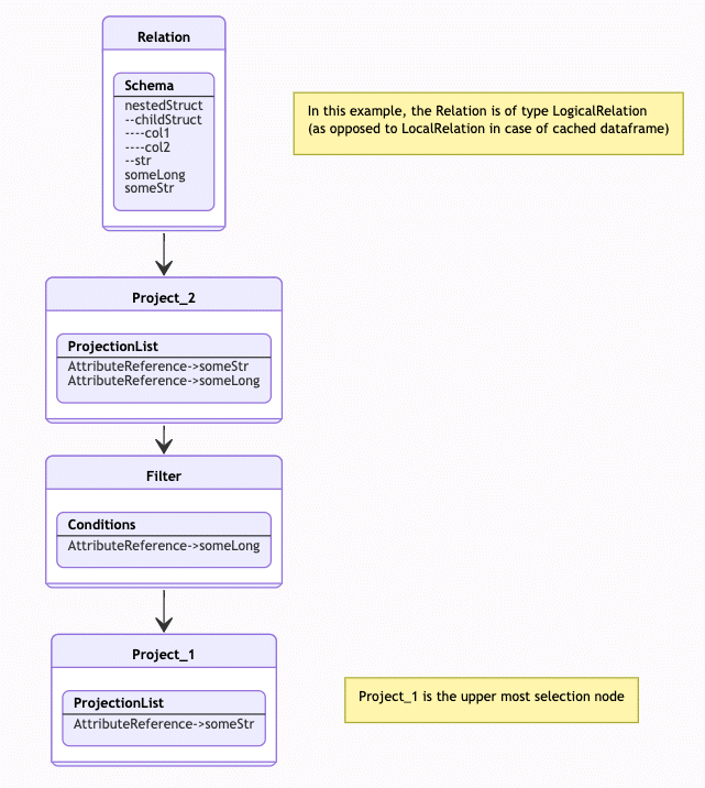
For each TreeNode in the LogicalPlan we apply different logic. For example, for the LogicalRelation, which holds an HadoopFsRelation, we store the relation reference in the state, and mark it as currentHadoopFsRelation.
Upon storing the relation reference, we also create a RelationSchema object for it, with full schema being the LogicalRelation schema of the underlying data, and an empty StructType for schema on read.
Moving on to the parent Project (Project_2 in Plan 1), we iterate the ProjectList and update the RelationSchema’s schema on read with the columns we identified.
In this case our partial schema would look like this:
root
 |-- someLong: long
 |-- someStr: string
Next, visiting the parent Filter, we iterate on the condition and update the RelationSchema with the newly observed columns. In this case, someLong is already present in schema, so there is nothing to update.
Finally, we get to the uppermost Project (Project_1), which already holds someStr, so again, no need to update..
Now that we’re done traversing the plan, we can use the created schema on read:
Dataset<Row> df = sparkSession.read().parquet(“/path/to/parquet”);
df = df.select(“someLong”, “someStr”)
.filter(“someLong = 5”)
.select(“someStr”);

StructType schemaOnRead = SchemaOnReadGenerator.generateSchemaOnRead(df).getSchemaOnRead(“/path/to/parquet”);
Dataset<Row> reducedSchemaDf = sparkSession.read().schema(schemaOnRead).parquet(“/path/to/parquet”);

// repeat the same query
reducedSchemaDf.select(“someLong”, “someStr”)
.filter(“someLong = 5”)
.select(“someStr”);
Notice that the schema on read for our DF is accessed by the path to the data. We have to assume there’s no single schema to be provided for the query, as the query might represent a join between several data sources, each with its own schema.
If we chose to provide an alias in the query, we also could have retrieved the schema by alias.
What Are You Implying?
Let’s review this simple Spark SQL query, but without the bottom project:
df.filter(“someLong = 5”)
.select(“someStr”)
While we didn’t explicitly instruct to select someLong in the scenario below, it’s implied by the filter node.
Plan 2 – field appears only in Filter node
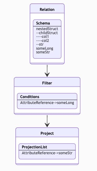
As we traverse the plan here, we again populate the schema on read for this query, but this time we only add someLong when we encounter the Filter, and then add someStr as we get to Project. The resulting schema is the same.
Things Are Complicated…
Let us consider a more tricky Spark SQL query with nested fields:
df.select(df.col(“nestedStruct”).as(“myStruct”))
.select(“myStruct.str”)
The LogicalPlan illustrated in Plan 3
Plan 3 – nested fields and aliases
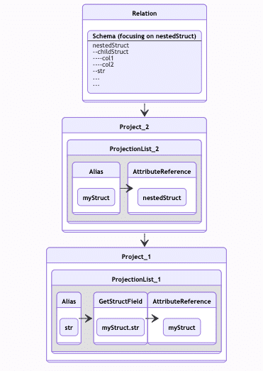
In Project_2 we query for nestedStruct. But we don’t really need the entire nestedStruct. In Project_1, we only take the str field from this nestedStruct. But to make things more complicated, we also have an alias for nestedStruct ?
We need to keep track of this alias, and exclude the redundant columns from the nestedStruct schema.
For each Relation we’re handling, we keep a map of SchemaElement objects. The SchemaElement can represent a concrete column from the relation schema, or it can represent a shadow instance of such a concrete SchemaElement, with the given alias. So when we encounter myStruct.str, we know that myStruct is an alias for nestedStruct, and that the str column is required.
Eventually, when deducing the required schema, we know that all we wanted from this nestedStruct is str, so we can toss the rest of its inner columns.
Another pleasant complication — given the above query, suppose we sort it by nestedStruct (even though it seems to make no sense).
df.orderBy(“nestedStruct”)
.select(df.col(“nestedStruct”).as(“myStruct”))
.select(“myStruct.str”)
Obviously, when we order by nestedStruct, we imply ordering by the entire content of it. If we had reduced our schema to have only nestedStruct.str, that would have changed the entire semantics of the query and yield incorrect results.
So how do we decide if we need the entire nestedStruct schema (for ordering), or just part of it (based on projection)?
We introduced the notion of conditional vs mandatory full schema. When visiting a TreeNode element while traversing the plan (see Plan 4), we mark whether the column requires the full schema (Sort node) or not (Project node). All of these attributes were taken into consideration while wrapping up the final schema on read.
Handling orderBy is also one of the most dangerous manipulations we can apply. Unlike many other clauses in queries, if we omit childStruct out of nestedStruct, we will not get a runtime exception, but we will get wrong results. So by all means, test coverage was one of the top most concerns in this project.
Plan 4 – Mandatory and conditional full schema

Even with these 4 examples, we have still only covered the tip of the iceberg. Things get more complicated with aggregations, window functions, explodes, array and map types etc.
Where trees are felled, chips will fly
ScORe is not flawless, it’s a best effort solution.
No doubt we have corner cases in which it will fail to generate a correct schema, or even fail to generate any schema. In fact, we do face such issues occasionally, and we address them as they come.
A classic example is a Spark SQL query that involves invoking a UDF on some column with a nested schema. The UDF is a blackbox, and so ScORe must assume we need the entire schema, even if the UDF needs only a subset of the schema.
There are other edge cases that we might encounter in production, as the syntax we support is mostly based on real production use cases. If tomorrow a developer or an analyst would use the PIVOT clause in a Spark SQL query, ScORe will probably fail.
As any other production code in Taboola, metrics are our eyes and ears. Nothing gets to production without proper visibility, and the scale of our metrics pipe alone (~100M distinct metrics per minute) is a BigData operation in itself.
At the Data Platform team, we also provide the infrastructure to execute Spark SQL queries over our data lake. ScORe is used by this infrastructure, so any query submitted, automatically benefits from it.
Normally a Spark SQL query is implemented as a Java class implementing the SqlQuery interface, and executed at least once an hour.
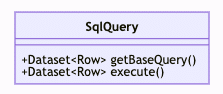
This interface includes the execute method that returns the DataFrame that we base the action on (normally saving the output to HDFS). Occasionally, the execute method itself is expensive even without performing an action. So we added the getBaseQuery method to the interface for the sake of ScORe, whereas the default implementation is just invoking execute.
When an SqlQuery implementation is first encountered, we use getBaseQuery to create the schema on read, and cache the result in memory. The price of generating the schema is ‘cheaper’ by several orders of magnitude compared to performing the action (and yes, we measure it as well).
We can then use the cached schema whenever we encounter the same SqlQuery implementation.
If we fail to generate a schema on read for a Spark SQL query, we are notified by alert. We also monitor for incompatible schemas. This might happen, for instance, if the query structure is based on some feature flag, and someone has changed its value. In this case, we would attempt to automatically regenerate the schema on read, and replace it in cache.
The getBaseQuery method is also useful when we face queries that SCoRe is not capable of handling properly. In the case of query using a UDF on a complex structure — we can use getBaseQuery to provide the exact columns from this complex structure and bypass this limitation.
For sql queries executed outside the scope of our datapipe infrastructures, developers can use ScORe directly in their code. For ad-hoc queries we’ve also modified zeppelins SparkSqlInterpreter to apply ScORe with a hint provided in the query.
Quod erat demonstrandum
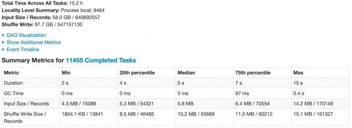
Recalling the production query we presented earlier, reading nearly 350GB of data.
Image 2 shows the effect of ScORe running the exact same Spark SQL query over exact same data.
Total input size has decreased to less than 60GB (nearly 85% reduction), and total time across tasks was reduced from 60 to 15 hours, WOW!
Image 2 – stats for stage reading input for production Spark SQL query using ScORe
With ~700 compute nodes running Spark jobs in our on-prem clusters, ScORe was a game changer. I hate to imagine the waste of resources if we did not develop this tool. And as an engineer, I’m lucky that the scale in Taboola constantly poses new challenges, forcing us to look for further optimizations.
At Spark, already significant progress was made for pruning nested schemas. These days we are working on upgrading our system to spark 3, so ScORe is still relevant to us as well as to anyone who is still using earlier spark versions. But even once we’re fully upgraded, pruning in spark 3 still doesn’t work for some syntax elements (e.g. window functions), so we expect ScORe to keep serving us for quite some time.
You are welcome to tweet us for any question!