Predicting Probability Distributions Using Neural Networks

If you’ve been following our tech blog lately, you might have noticed we’re using a special type of neural networks called Mixture Density Network (MDN). MDNs do not only predict the expected value of a target, but also the underlying probability distribution.

This blogpost will focus on how to implement such a model using Tensorflow, from the ground up, including explanations, diagrams and a Jupyter notebook with the entire source code.

What are MDNs and why are they useful?

Real life data is noisy. While quite irritating, that noise is meaningful, as it gives a wider perspective of the origins of the data. The target value can have different levels of noise depending on the input, and this can have a major impact on our understanding of the data.

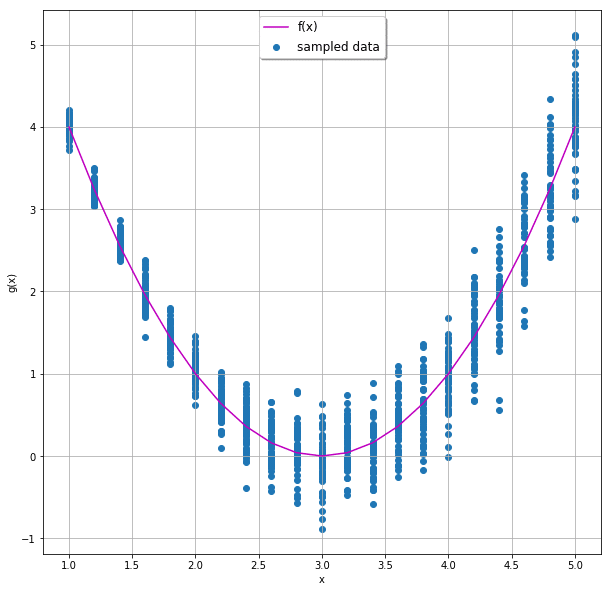
This is better explained with an example. Assume the following quadratic function:

Let’s sample g(x) for different x values:

The concept of MDN was invented by Christopher Bishop in 1994. His original paper explains the concept quite well, but it dates back to the prehistoric era when neural networks weren’t as common as they are today. Therefore, it lacks the hands-on part of how to actually implement one. And so this is exactly what we’re going to do now.

Let’s get it started

Let’s start with a simple neural network which only learns f(x) from the noisy dataset. We’ll use 3 hidden dense layers, each with 12 nodes, looking something like this:

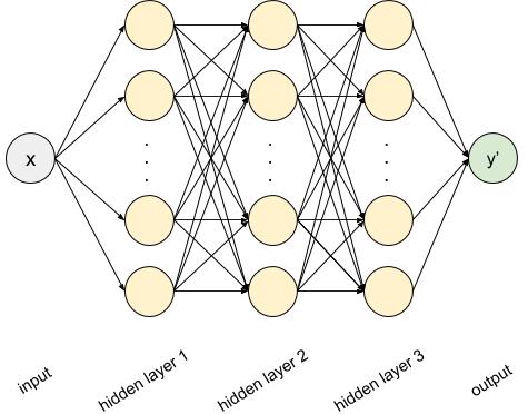
x = tf.placeholder(name='x',shape=(None,1),dtype=tf.float32)
layer = x
for _ in range(3):
   layer = tf.layers.dense(inputs=layer, units=12, activation=tf.nn.tanh)
output = tf.layers.dense(inputs=layer, units=1)

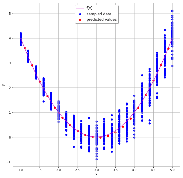
After training, the output looks like this:

Going MDN

We will keep on using the same network we just designed, but we’ll alter two things:

1. The output layer will have two nodes rather than one, and we will name these mu and sigma
2. We’ll use a different loss function

Now our network looks like this:

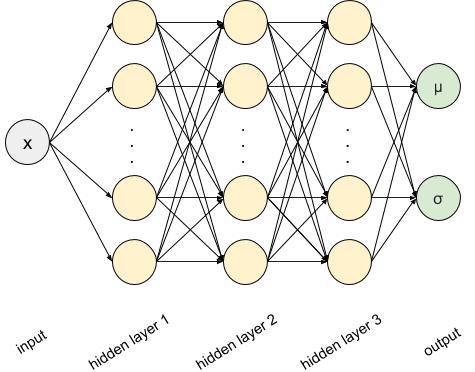
x = tf.placeholder(name='x',shape=(None,1),dtype=tf.float32)
layer = x
for _ in range(3):
   layer = tf.layers.dense(inputs=layer, units=12, activation=tf.nn.tanh)
mu = tf.layers.dense(inputs=layer, units=1)
sigma = tf.layers.dense(inputs=layer, units=1,activation=lambda x: tf.nn.elu(x) + 1)

Let’s take a second to understand the activation function of sigma – remember that by definition, the standard deviation of any distribution is a non-negative number. The Exponential Linear Unit (ELU), defined as:

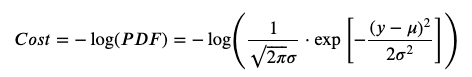
Next, we need to adjust our loss function. Let’s try to understand what exactly we are looking for now. Our new output layer gives us the parameters of a normal distribution. This distribution should be able to describe the data generated by sampling g(x). How can we measure it? We can, for example, create a normal distribution from the output, and maximize the probability of sampling our target values from it. Mathematically speaking, we would like to maximize the values of the probability density function (PDF) of the normal distribution for our entire dataset. Equivalently, we can minimize the negative logarithm of the PDF:

dist = tf.distributions.Normal(loc=mu, scale=sigma)
loss = tf.reduce_mean(-dist.log_prob(y))

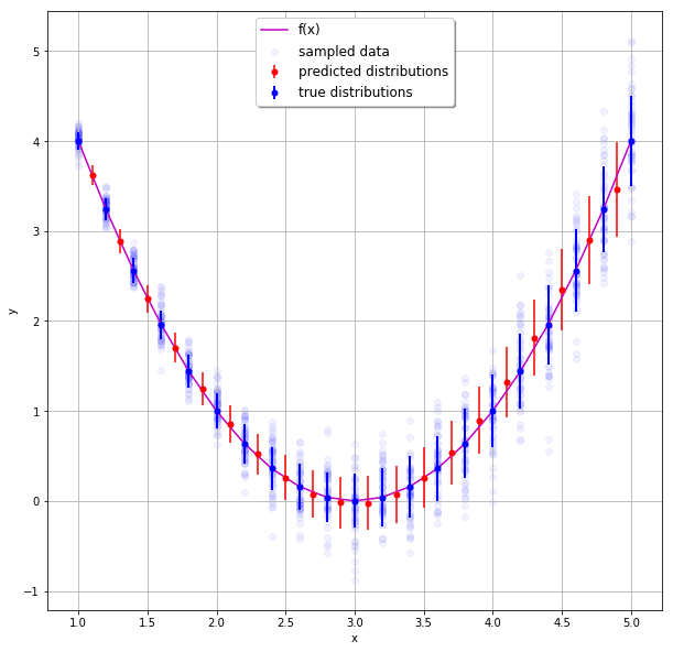
And that’s about it. After training the model, we can see that it did indeed pick up on g(x):

Next steps

We’ve seen how predict a simple normal distribution – but needless to say, MDNs can be far more general – we can predict completely different distributions, or even a combination of several different distributions. All you need to do is make sure to have an output node for each parameter of the distribution’s variables, and validate that the distribution’s PDF is differentiable.

I can only encourage you to try and predict even more complex distributions – use the notebook supplied with this post, and change the code, or try your new skills on real life data! May the odds be ever in your favor.