Taboola is responsible for billions of daily recommendations, and we are doing everything we can to make those recommendations fit each viewer’s personal taste and interests. We do so by updating our Deep-Learning based models, increasing our computational resources, improving our exploration techniques and many more. All those things though, have one thing in common – we need to understand if a change is for the better or not, and we need to do so while allowing many tests to run in parallel.
We can think of many KPI’s for new algorithmic modifications – system latency, diversity of recommendations or user-interaction to name a few – but at the end of the day, the one metric that matters most for us in Taboola is RPM (revenue per mill, or revenue per 1,000 recommendations), which indicates how much money and value we create for our customers on both sides – the publishers and advertisers. RPM can get a little noisy – it is influenced by external factors such as current events (how interesting the news is right now) or time of year (aren’t we all waiting for the holidays?) but also by internal factors such as system upgrades and our own experiments – which can affect one another and add extra noise to the mix. All those mean that RPM can change by as much as 5-10% from day to day. But an algorithmic improvement, on the other hand, might be even lower than 1%. So how can we tell if a change is for the better? All it takes is proper data handling and some pretty basic statistics.
The Simpsons
Let’s start with data handling. With the enormous amount of data we handle at Taboola, you can rest assured that we’ve seen many interesting phenomena that caused us to scratch our heads. For instance, take a look at the data in the table below, which shows how well two variants are doing on a four day period. If you look carefully you’ll see that in each of the 4 days, the test variant has higher RPM values than the default variant. However, when aggregating results from all 4 days the default variant all of the sudden has a higher RPM. This brings up two questions:
- How is that possible?
- Is the test variant winning or losing?
| default variant | test variant | |||||
| date | RPM | count | revenue | RPM | count | revenue |
| 2020-05-01 | 1.358 | 123,651,344 | 167,896 | 1.399 | 41,385,732 | 57,888 |
| 2020-05-02 | 1.190 | 157,182,560 | 186,992 | 1.200 | 77,811,946 | 93,370 |
| 2020-05-03 | 1.068 | 151,712,429 | 161,976 | 1.075 | 74,929,584 | 80,538 |
| 2020-05-04 | 0.988 | 141,997,417 | 140,288 | 0.995 | 70,248,390 | 69,864 |
| Grand Total | 1.144 | 574,543,750 | 657,152 | 1.141 | 264,375,652 | 301,661 |
Table 1: Daily stats for two variants over the course of 4 days
First off, this is not only possible, but can actually happen quite often. This phenomenon is called “Simpson’s paradox”, where combining several groups together cancels out a trend that appears individually in each group (you can read more on Simpson’s Paradox here). The answer to the second question is hidden in the first day – take a close look at the second table below, which presents the traffic counts for each variant and the ratio between them:
| date | default count | test count | count ratio |
| 2020-05-01 | 123,651,344 | 41,385,732 | 0.33 |
| 2020-05-02 | 157,182,560 | 77,811,946 | 0.50 |
| 2020-05-03 | 151,712,429 | 74,929,584 | 0.49 |
| 2020-05-04 | 141,997,417 | 70,248,390 | 0.49 |
| Grand Total | 574,543,750 | 264,375,652 | 0.46 |
Table 2: Comparing the number of recommendations each variant had
It can be seen that in the first day of the experiment, the ratio is way off (0.33 compared to 0.49-0.5 on other days). Looking closely into the matter we found out that we included the day of the variant setup in the experiment, so it was a full day for the default variant and a partial day for the test variant. Because the first day happened to be the most profitable day by far (check out the RPM columns in the first table), and because the test variant got a smaller chunk of it, its overall measure was lower even though it had better measures on all 4 days. What we learn from this example is that taking a look at the traffic split between variants, and making sure it is consistent, is important if we wish to avoid strange skews in the data. Our testing procedure in Taboola tests for such cases and others, and gives the researcher a green light if the experiment is winning with confidence, a red light if it is losing with confidence and an alert if some issues were found that need a closer look.

It’s T-Time
And how exactly do we gain this confidence? This brings us to the statistical part of this blogpost, or more specifically, to a paired sample t-test.
Paired sample t-test is used when we can match each observation from one sample to an observation from the other. For our case we use the daily average revenue as a single data point, and the pairing is done over days. This means that for each variant we have a sequence of numbers and just like a normal t-test, we try to reject the null hypothesis:
: The means of the test variant RPM and default variant RPM are equal
But while a normal t-test goes like this:
( and
are the unbiased estimators for the sample mean and sample variance respectively)
A paired sample t-test goes like this:
The great advantage of the paired sample t-test over the normal t-test is that it allows us to cancel the time related noise and focus on the difference between the two variants. For example, take a look at the results given in the following figure: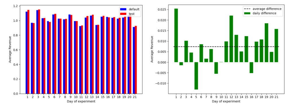
Figure 1: Left: average revenue (per recommendation) of two variants over the course of 21 days
Right: the difference in the average revenue along the same 21 days
Using the normal t-test to compare the two variants, we get a p-value of ~0.7, which means we have about 30% confidence in rejecting the null hypothesis that the two variants have equally distributed means. This happens because the difference between days is much greater than the average difference between test and default. However, using the paired sample t-test yields a p-value of ~0.001, or 99.9% confidence in rejecting our null hypothesis (I will not dive into the subtleties of the confidence term, let’s keep it simple). If you need more intuition as to why the paired sample t-test improves the confidence to such an extent, compare the figure above to the one below – which shows a permutation of the days for test and default data such that we can no longer pair by days. In a sense, the un-paired t-test uses the data representation below while the paired t-test uses the data representation above.

Figure 2: Same test and default variants, but this time days are permuted randomly so that pairing is not known
Whenever using a statistical test, it is important to ask ourselves if it’s the right one. In our case, we made sure our data meets these 3 requirements for using a t-test:
- The sample means for both populations are normally distributed. For large samples this assumption is met due to the central limit theorem, but for smaller samples this needs to be tested. We use daily aggregated data so our sample is as big as the amount of days in the experiment, which is typically not very large. To test this requirement, we used the Shapiro-Wilk normality test and got good results.
- The two samples have the same variance. This is only required when the samples are not of equal size. We have equal size samples, and t-test is very robust to cases with unequal variance, so no worries there.
- The sampling should either be entirely independent or entirely paired. Our daily data is linked through the general behavior on each day, which means we need to perform a paired test, and that is exactly what we did.
Final Words
When we are testing new variants of our system we face contradicting interests. On the one hand, we want to make decisions fast – removing losing variants quickly and diverting more traffic to the winning ones yields greater value. On the other hand, the more time we give our variants, the more certainty we have in their performance, reducing the chance of making wrong decisions. This post gives a peek at how we use some pretty basic statistical principles and combine them with general “know-hows” of data handling in order to balance those interests, and make sure we gain as much information as possible from the time we give our variants. Have any thoughts? Let us know!